
Comparison of Grouped Aggregate Queries
First Published 3 Jan 2023 Last Updated 6 Jan 2023 Difficulty level : Moderate
Section Links:
Introduction
The Task
Tests / Results
Query Execution Plans
Query Execution Plans - Summary
Additional Tests / Results
Yet More Tests / Results
Conclusions
Download
Further Reading
Feedback
1. Introduction Return To Top
This is the fifteenth in a series of articles discussing various tests done to compare the efficiency of different approaches to coding.
In this article, the efficiency of 5 different types of aggregate query are compared including the use of non equi-joins and subqueries.
Unexpectedly, it then led into a long investigation into the effects of indexing in aggregate queries.
The article was inspired by a suggestion from fellow Access developer Chris Arnold at the end of my presentation on Optimising Queries to the online
Access Europe User Group in September 2022
You can watch the YouTube video of that presentation at
https://www.youtube.com/watch?v=mVe3InnJaAE
2. The Task Return To Top
Using DEMO data from my main schools database:
Count the number of reading age (RA) tests (where >1) for each student that were a lower RA value than the most recent test.
This is a simplified version of a real situation from my own school where the Special Educational Needs (SEN) department was required to provide a range of
reports indicating the amount of intervention for students done over a period of time.
The original version of this query gave the data obtained for one such test.
Four other versions of the same query have also been tested here for comparison
The 2 tables used here are cut down versions of the original SQL Server tables with dummy data
PupilData (PD)
1482 records; 9 fields; Indexes - PupilID (PK text), Surname+Forename (composite text), Reading (text)
SENTestHistory (TH)
4946 records; 5 fields; Indexes – SENTestHistoryID (PK autonumber), PupilID (FK text), Type (text), Level (text)
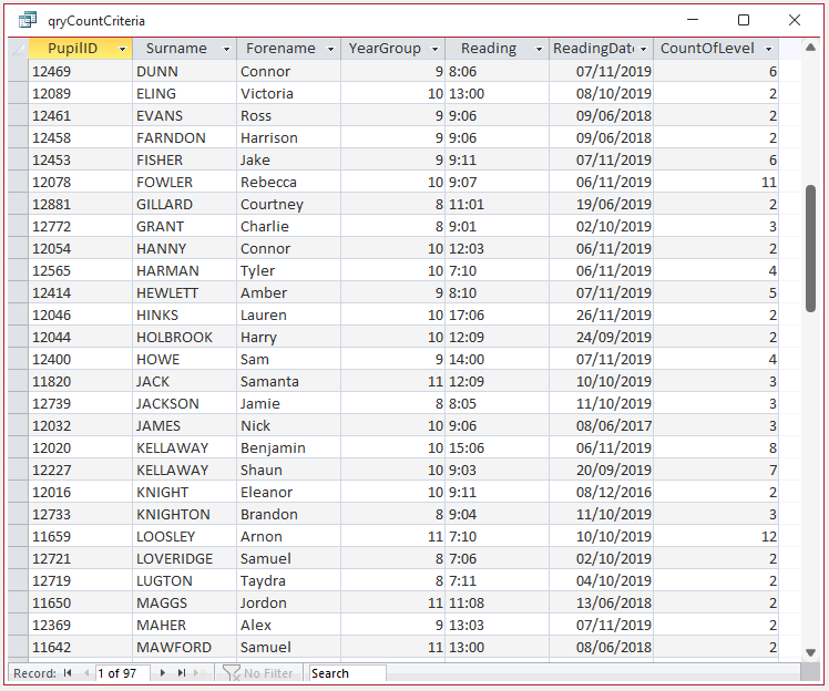
Query Output:
97 records, 7 fields (for all 5 queries)
This is part of the aggregated query output from one of the queries. All 5 queries have been designed to provide the same output
NOTE:
Reading age is expressed in years:months e.g. 13:07. Students take targeted tests aimed at a certain range e.g. 9:03 to 11:09
Where a result is outside the limits for that test, values may be expressed as e.g. 9:03- or 11:09+
In such cases, the student would be re-tested using a different test range
Similar tests are done to measure the Spelling age and Arithmetic age and are also used to focus targeted support on those students with greatest need.
Each test result is stored in the Level field of the SENTestHistory table.
For historical reasons, the most recent test result is also recorded in the Reading field of the PupilData table.
The five queries used in these tests were as follows:
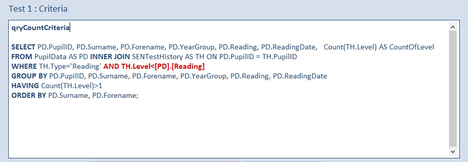
a) qryCountCriteria
This is a standard grouped aggregate query on the two tables using an INNER JOIN with 2 WHERE filters and a HAVING filter on the aggregate field
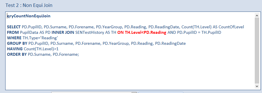
b) qryCountNonEquiJoin
In this query, the unequal WHERE filter is replaced by a non-equi join. This query must be saved in SQL view
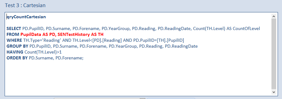
c) qryCountCartesian
In this query, the tables are not joined. All filtering is done using the WHERE and HAVING clauses
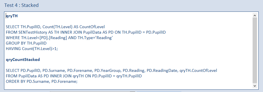
d) qryCountStacked
Here an aggregate query qryTH is used to get the aggregate values then this is joined to the PupilData table in qryCountStacked
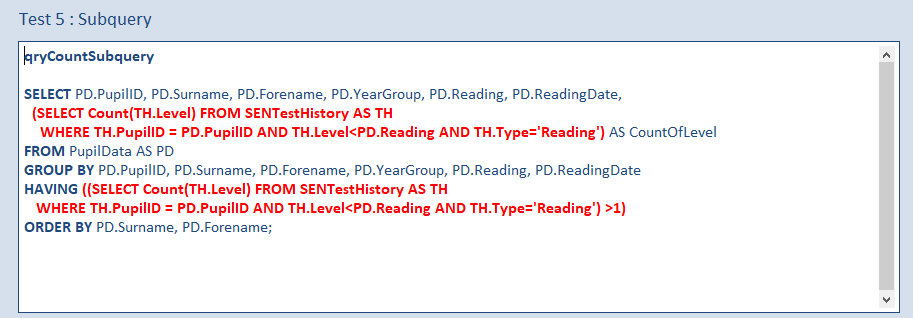
e) qryCountSubquery
A subquery is used to get the aggregate values so no table joinis needed in the main query. The HAVING clause references the subquery.
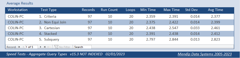
3. Tests / Results Return To Top
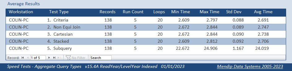
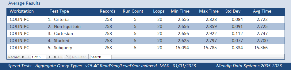
Each test consisted of the queries being run 20 times in succession and the total time measurered.
Each test was repeated 10 times in a random order and the average times calculated.
The first 4 tests were very similar with the criteria query the fastest and the cartesian query the slowest. This was exactly as I had expected.
However, the differences between these 4 queries was minimal.
I had expected the subquery version to be slower but not that it would take about 10 times longer! This was VERY surprising.
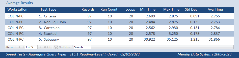
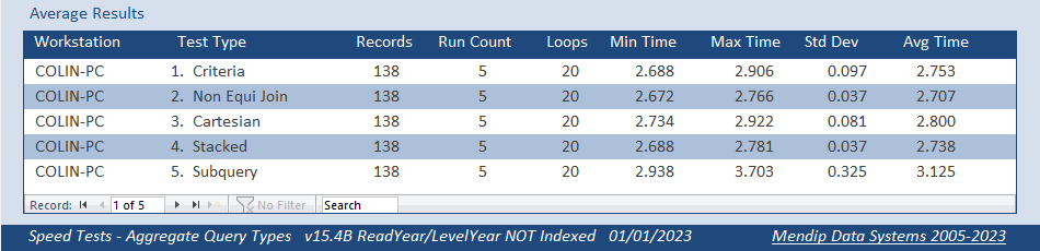
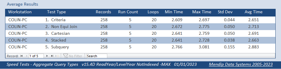
I removed the index from the Level field used in aggregation.
The first 4 queries were slightly faster with the overall order remaining the same.
However, there was a significant improvement for the subquery version which, although still the slowest, was now only about 14% slower
I then also removed the index from the Reading field in the PupilData table with which the Level is compared in the filter.
Once again, the overall order remained unchanged. However, doing this took about 0.3 to 0.35 s off each time
Overall, the standard query based on a table join and WHERE/HAVING criteria is the most efficient in these tests.
I was surprised how well the cartesian query performed
However, there are two obvious questions arising from these tests:
a) Why did REMOVING the indexes speed up all the queries?
b) Why does indexing have such a large adverse effect on the subquery performance?
To investigate each of these, I carried out a large number of additional tests
4. Query Execution Plans Return To Top
I compared the query execution plans (QEP) using the hidden, undocumented JET ShowPlan feature. See my article: Show Plan . . . Go Faster
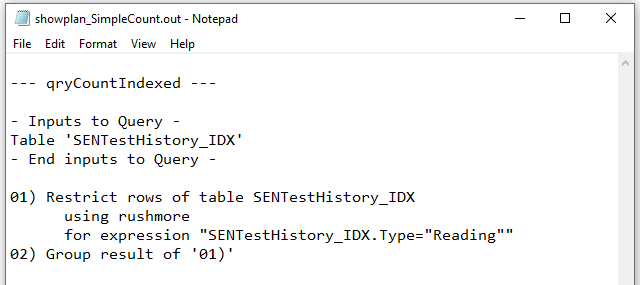
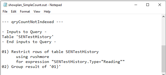
a) First of all, as a benchmark, I ran a grouped aggregate query on the SENTestHistory table alone with the Level field indexed then not indexed.
The query SQL for each was:
SELECT TH.PupilID, Count(TH.Level) AS CountOfLevel
FROM SENTestHistory AS TH
WHERE TH.Type="Reading"
GROUP BY TH.PupilID
HAVING Count(TH.Level)>1;
The results showed that there was almost no difference between the times for each version.
The query execution plans were as follows:
Level Field Indexed
|
Not Indexed
|
Both QEPs were identical. The index on the Type field was used in each case and Rushmore query optimising technology was involved.
I repeated the tests on a much larger table of student attendance marks with about 680K records.
Once again, indexing had minimal effect on the times to run a grouped aggregate query on a single table
This suggests the explanation for the differences shown in the original set of results must lay elsewhere.
Next I compared the query execution plans for the 5 types of grouped aggregate query tested above
b) qryCountCriteria
Both Fields Indexed
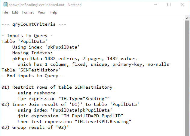
|
Not Indexed
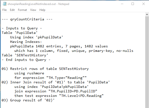
|
Both QEPs were again identical. The available indexes were used in each case and Rushmore query optimising technology was involved.
c) qryCountNonEquiJoin
Both Fields Indexed
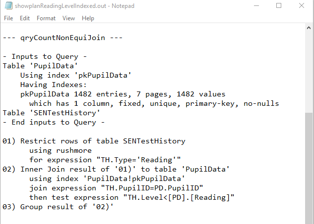
|
Not Indexed
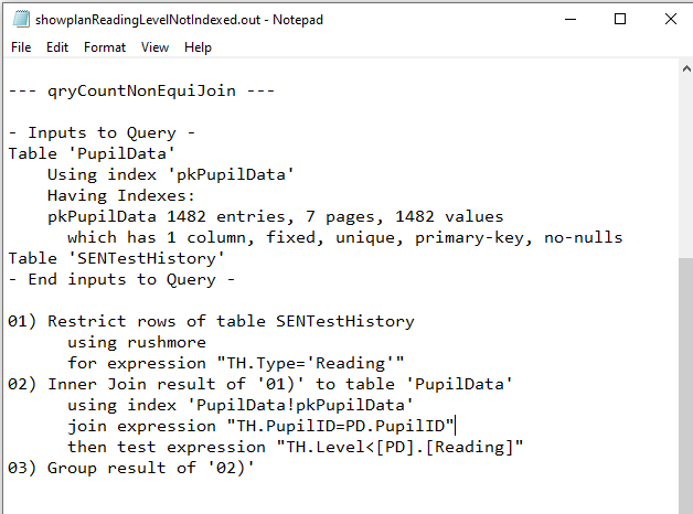
|
Both QEPs were again identical. Same comments as above
d) qryCountCartesian
Both Fields Indexed
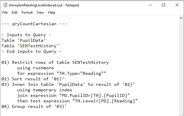
|
Not Indexed
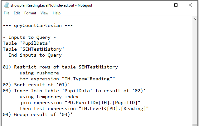
|
Yet again, both QEPs were identical. Rushmore used on the SENTestHistory table with a temporary index on the PupilData table
e) qryCountStacked
Both Fields Indexed
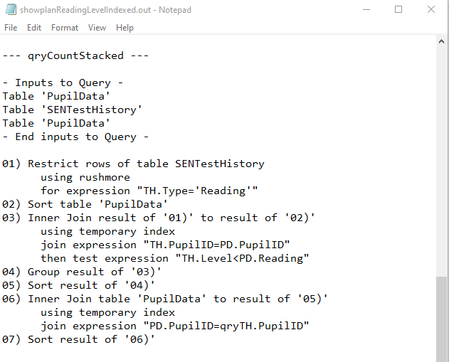
|
Not Indexed
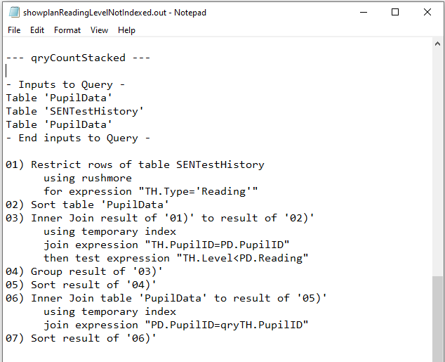
|
Yet again, both QEPs were identical. Rushmore used on the SENTestHistory table with two sets of temporary index on the PupilData table
f) qryCountSubquery
Both Fields Indexed
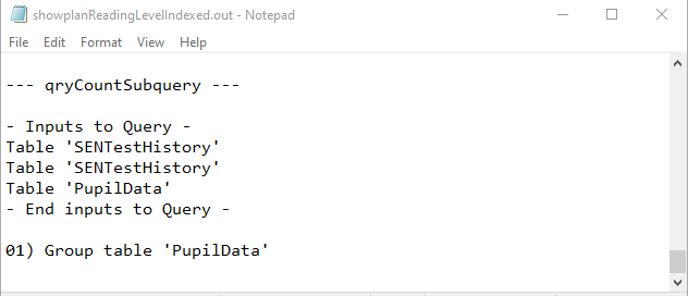
|
Not Indexed
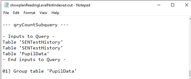
|
Yet again, both QEPs were identical.
Unfortunately JET ShowPlan does NOT give the execution plans for subqueries
However, there is no mention of Rushmore being used elsewhere in the final query.
That alone almost certainly makes the subquery less efficient i.e. slower.
5. Query Execution Plans - Summary Return To Top
The first 4 queries all used the available indexes effectively with Rushmore query optimisation technology utilised for sorting and filtering.
However, each of the QEPs were identical when the queries were run with the two indexes used in aggregation removed.
So that explains why the order is unchanged.
However, it does not explain why each query ran slower when indexed nor why the subquery was so adversely affected by the indexes
The Microsoft help article: Create and use an index to improve performance states that you should consider indexing a field if all of the following apply:
a) The field's data type is Short Text, Long Text, Number, Date/Time, AutoNumber, Currency, Yes/No or Hyperlink.
b) You anticipate searching for values stored in the field.
c) You anticipate sorting values in the field.
d) You anticipate storing many different values in the field. If many of the values in the field are the same, the index might not significantly speed up queries.
As a check, I compared the table index statistics:
PupilData: Records = 1482; Unique Index Values (Reading Field) = 99 (approx 6.6% of number of records)
SENTestHistory: Records = 4946; Index Values (Reading Field) = 138 (approx 2.7% of number of records)
In my opinion, that should have made both fields well suited to indexing in this example
6. Additional Tests / Results Return To Top
As a further test, I altered the reading age data in both tables to only show the years as an integer value
e.g. 7:11 => 7; 14:05 => 14 giving a range from 5 to 18
NOTE: This was done just for the purpose of testing here. It would be of very little use for educational purposes
Doing this reduced the number of unique indexed values to just 14 for the aggregated Level field and 13 for the Reading field in the PupilData table
There were now 138 records returned by each query but the pattern was much the same as before
Both fields indexed
Both fields NOT indexed
So it appears that the size of the original indexes wasn't the issue!
Although I had no reason to suspect that using Count was an issue, I decided to eliminate it by using a different aggregate function Max rather than Count
Both fields indexed
Both fields NOT indexed
Different values but same trend again . . .
I also tested with the same data in linked SQL tables from the original dataset
The first 4 queries were much the same as before but the subquery was many times slower still!
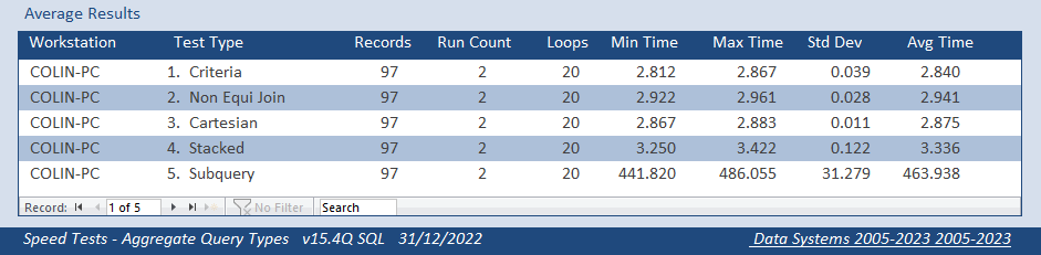
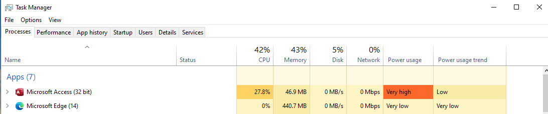
Whilst running the subquery, the task manager showed high CPU, memory and power usage
I now went back to the original dataset and started altering the criteria used in each query
First of all, I removed the restriction that there had to be more than one result in the Count(Level) aggregate field.
As a result there were now more records - 195 in total
Both fields indexed
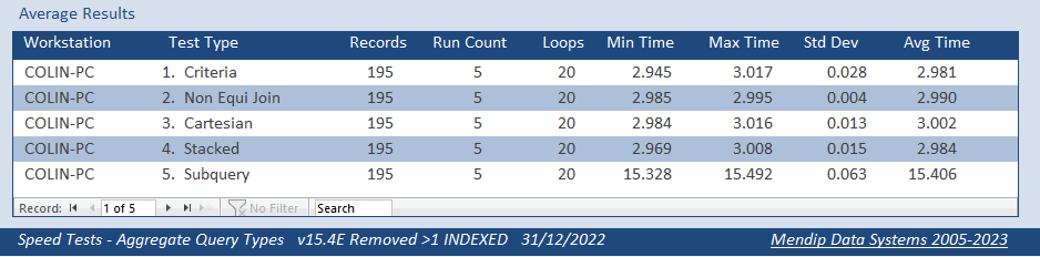
Both fields NOT indexed
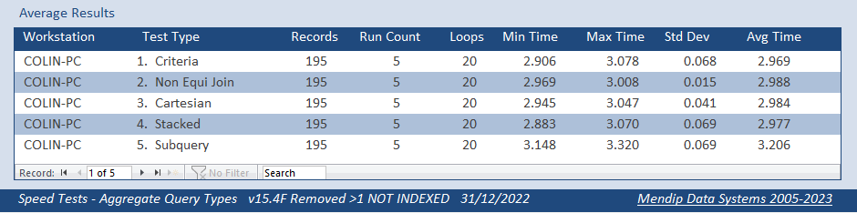
Finally, with the exception of the subquery, the indexed versions all took about the same time as their non-indexed equivalent.
The subquery took about 16s. That was about half the original time for the indexed field
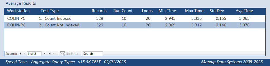
Next, I removed the restriction that the values counted in the Level field had to be less than the latest value in the Reading field.
As a result there were now more records - 329 in total
I discarded the non equi-join query as this was no longer relevant
Both fields indexed
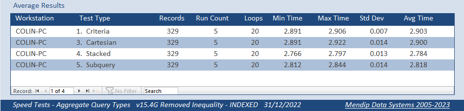
Both fields NOT indexed
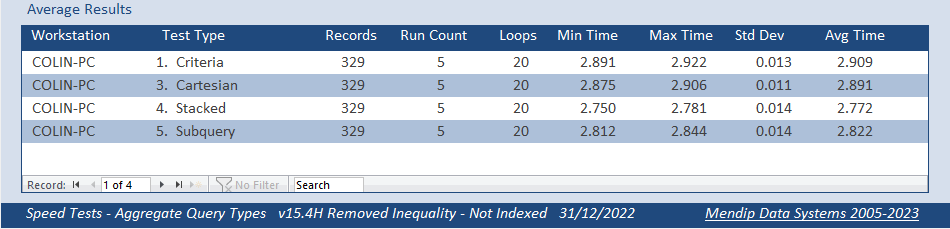
BINGO! The indexed and non-indexed versions of each query were now very similar in terms of the time taken
The subquery was no longer the slowest, only being beaten by the stacked query
I decided to do one further test removing both sets of restrictions.
The number of records was now 1423 and included almost all the students in the dataset.
Both fields indexed
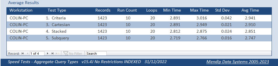
Both fields NOT indexed
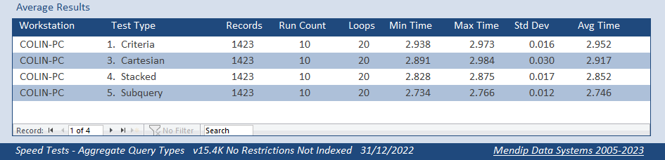
Again, both sets of tests took almost exactly the same time. Indexing was no longer harmful, but it still offered no benefit.
However, to my surprise, the subquery was now the fastest method of all taking about 5% LESS time than the other 3 queries.
To me, this was remarkable!
It is the very first time in 20+ years of using Access that I have EVER seen a subquery outperform a well optimised single query
The charts below compare the relative speeds of all the queries in the original non-indexed test to the final non-indexed test.
As you can see, the order is almost exactly reversed in the final simplified tests.
Of course, the vertical axis scale 'over dramatises' the time differences.
Original Query
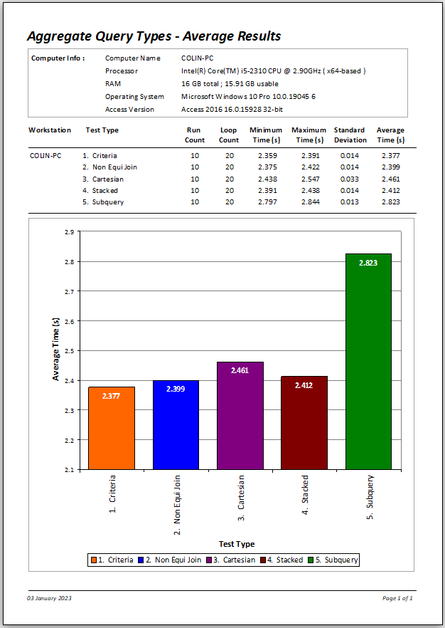
|
Final Query
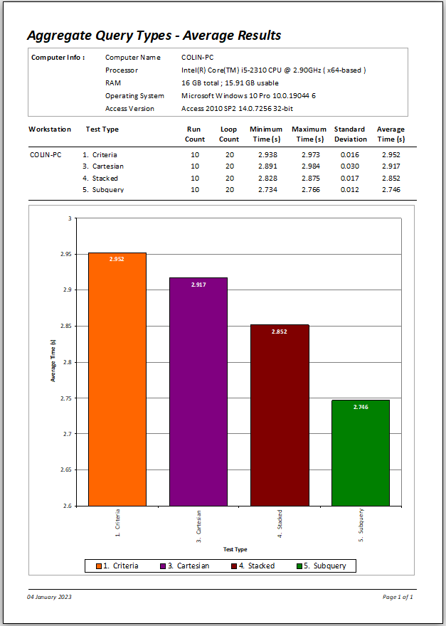
|
Unfortunately, the query designs were by now so simple that the query output was totally useless for the original purpose!
Finally, I looked at the QEPs again for the final set of queries used above
By now, it probably won't surprise you that in each case the QEPs were again identical for the indexed and non-indexed versions!
Not only that, but they were effectively identical to those for the original set of queries.
The only difference was that the order of events did change slightly for the stacked query, but the actual steps were exactly the same.
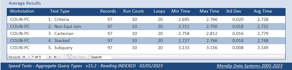
7. Yet More Tests / Results - UPDATE 5 Jan 2023 Return To Top
After publishing this article, I decided to try one more set of tests.
On a hunch, I decided to go back to the original query, retain both indexes on the Level and Reading fields, but force Access to ignore them.
To remind you, these were the original results with both fields indexed
And these were the original much faster results with both indexes removed
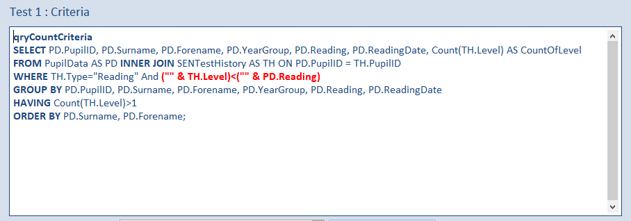
In order to ignore the indexes, I just added an zero length string to the start of both fields used in the inequality filter.
In other words, I changed the inequality used in each query from: TH.Level < PD.Reading to ("" & TH.Level) < ("" & PD.Reading)
For example, qryCountCriteria:
After making this change, these were the new average results:
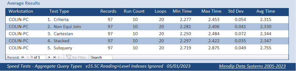
SUCCESS!!!!! All 5 queries ran faster than before with the standard criteria query being fastest and the subquery remaining slowest.
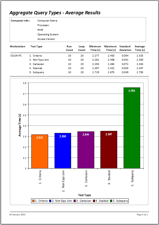
We now have the best of both worlds! The queries were for the original task with both indexes included but ignored for the inequality filter.
Also, as you probably expect by now, the query execution plans were almost identical to before, apart from the use of the changed inequality.
The one exception was that the Cartesian query made better use of indexing
8. Conclusions Return To Top
The use of indexes on suitable fields is generally beneficial in speeding up searches and sorts.
However, it appears to offer no benefit on the fields used in aggregate queries.
In many cases, indexing the fields used in aggregation (or compared with them) can make grouped aggregate queries run noticeably slower.
Despite this, retaining the indexes but ignoring them in the inequality filter proved the most efficient method of all.
In general, the standard grouped aggregate query involving joins and where criteria performs as well as any of the other more unusual variants.
Using a subquery in aggregation is generally a bad idea unless the query has no conditions/restrictions associated with the aggregated field
NOTE: In the near future, I plan to do two follow up articles provisionally called The Art of Indexing and The Joy of Subqueries !!!!
EDIT: 6 Jan 2023
Perhaps some additional clarification is needed following a lengthy critique of this article by @ebs17 at Access World Forums
This article was intended purely as a comparison of 5 different types of grouped aggregate query.
At no time have I implied that any of the queries are fully optimised.
There are several further improvements that can be made including the use of First vs Group By that was discussed in my earlier article Optimising Queries
There is also an issue with the inequality filter though this doesn't affect the comparative speed tests.
However, this article is already far longer than originally intended due to the lengthy digression on the effects of indexing.
I am intending to return to all these points as part of my forthcoming article devoted to indexing.
9. Download Return To Top
Click to download the example databases with all code used in these tests. The query execution plans are also included in each zip file.
Comparing Aggregate Queries - INDEXED Approx 2.1 MB (zipped)
Comparing Aggregate Queries - NOT INDEXED Approx 2.1 MB (zipped)
Comparing Aggregate Queries - INDEXES IGNORED Approx 2.1 MB (zipped)
10. Further Reading Return To Top
I have not been able to find anything online explaining the effect of indexing on aggregate queries or why it disproportionately affects subqueries in Access
Here is a generic Microsoft help article about indexing
Create and use an index to improve performance
Here is an interesting article about indexing in SQL Server
Poor database indexing – a SQL query performance killer – recommendations
11. Feedback Return To Top
Please use the contact form below to let me know whether you found this article interesting/useful or if you have any questions/comments.
Please also consider making a donation towards the costs of maintaining this website. Thank you
Colin Riddington Mendip Data Systems Last Updated 6 Jan 2023
Return to Speed Test List Page 15 1 2 3 4 5 6 7 8 9 10 11 12 13 14 15 Return to Top
|
|
|